Dynamic Neural Fields

The dynamical neural field (DNF) theory has been introduced by Wilson and Cowan, and latter formalised by Amari and Taylor. This theory considers a neural population at the tissue level governed by a unique differential equation that describe the spatio-temporal evolution of coarse grained variables such as synaptic or firing rate activity. There have been numerous theoretical works related to the study of DNF properties like pattern formation, analytical solution, bifurcation conditions, etc.

More formaly, DNF equation reads:

1/α ∂u(x,t)/∂t = -u(x,t) + ∫ w(║y-x║) f(u(y,t))dy + I(x,t) (1)

where:

• u(x,t) is the potential of neural population at position x and time t
• w(d) is a neighborhood function from ℝ→ℝ
• f(u) is the firing rate of a single neuron
• α is the temporal decay of the synapse
• I(x,t) is the input at position x.

It is thus straightforward to numerically integrate the equation considering a given spatial and temporal resolution.

n = 256
src = np.zeros((n,))
tgt = Group((n,), """ dU/dt = (-V + 0.1*L + I);
                          V = maximum(U,0);
                          I; L """)
SparseConnection(src, tgt('I'), np.ones((1,)))
SharedConnection(tgt('V'), tgt('L'), +1.10*gaussian(2*n+1, 0.20)
                                     -0.95*gaussian(2*n+1, 1.00))

Gray Scott reaction-diffusion model

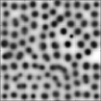
The Gray Scott model is a mathematical model of the reaction and diffusion of chemical species and may produce a variety of behaviors as illustrated below:

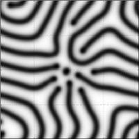
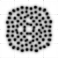
A Gray Scott model is described by a set of two differential equations:

• ∂u/∂t = Du ∇²u - uv² + f(1-u) (1)
• ∂v/∂t = Dv ∇²v + vu² - (f+k)v (2)

that can be very easily modeled using DANA:

Z = Group((n,n), """ du/dt = Du*Lu - Z + F*(1-U)
                     dv/dt = Dv*Lv + Z - (F+k)*V
                     U = np.maximum(u,0)
                     V = np.maximum(v,0)
                     Z = U*V*V
                     Lu; Lv; """)
K = np.array([[np.NaN,  1., np.NaN],
              [  1.,   -4.,   1.  ],
              [np.NaN,  1., np.NaN]])
SparseConnection(Z('U'),Z('Lu'), K, toric=True)
SparseConnection(Z('V'),Z('Lv'), K, toric=True)

The full sources for screenshots above are available from the models directory in the DANA distribution.

Bellman-Ford algorithm

The Bellmann-Ford algorithm can be implemented using DANA as illustrated below:

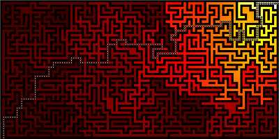
The idea is simply to use DANA to diffuse a value and to climb back the V value to get the shortest path.

n = 61
a = 0.99
Z = 1-maze((n,2*n+1))
G = Group((n,2*n+1),'''V = I*maximum(maximum(maximum(maximum(V,E),W),N),S)
                       W; E; N; S; I''')
SparseConnection(Z, G('I'), np.array([ [1] ]))
SparseConnection(G('V'), G('N'), np.array([ [a],      [np.NaN], [np.NaN] ]))
SparseConnection(G('V'), G('S'), np.array([ [np.NaN], [np.NaN], [a]      ]))
SparseConnection(G('V'), G('E'), np.array([ [np.NaN,  np.NaN,  a]        ]))
SparseConnection(G('V'), G('W'), np.array([ [a,       np.NaN,  np.NaN]   ]))