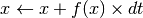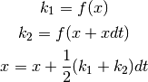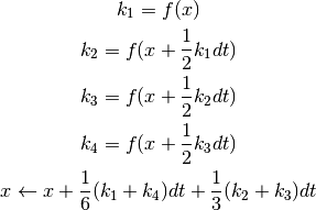
Differential equations may be solved using several methods that can be selected with the DifferentialEquation.select() method of the differential equation object. Below is the description of each method.
Most computational paradigms linked to artificial neural networks (using rate
code) or cellular automata use implicitly what is called synchronous evaluation
of activity. This means that information at time t+dt is evaluated exclusively
on information available at time t. The explicit numerical procedure to perform
such a synchronized update is to implement a temporary buffer at the unit level
where activity computed at time  is stored. Once all units have
evaluated their activity at time , The current activity is
replaced by the content of the buffer. We point out that other update
procedures have been developed [Lambert:1991] but the basic idea remains the
same, namely not to mix information between time
is stored. Once all units have
evaluated their activity at time , The current activity is
replaced by the content of the buffer. We point out that other update
procedures have been developed [Lambert:1991] but the basic idea remains the
same, namely not to mix information between time  and time
  . To perform such a synchronization, there is thus a need for a global signal
that basically tell units that evaluation is over and they can replace their
previous activity with the newly computed one. At the computational level, this
synchronization is rather expensive and is mostly justified by the difficulty
of handling asynchronous models.
. To perform such a synchronization, there is thus a need for a global signal
that basically tell units that evaluation is over and they can replace their
previous activity with the newly computed one. At the computational level, this
synchronization is rather expensive and is mostly justified by the difficulty
of handling asynchronous models.
For example, cellular automata have been extensively studied during the past decades for the synchronous case and many theorems has been proved in this context. However, some recent works on asynchronous cellular automata showed that the behavior of these same models and associated properties may be of a radical different nature depending on the level of synchrony of the model (you can asynchronously evaluate only a subpart of all the available automata). In the framework of computational neuroscience we may then wonder what is the relevance of synchronous evaluation since most generally, the system of equations is supposed to give account of a population of neurons that have no reason to be synchronized (if they are not provided with an explicit synchronization signal).
In [Taouali:2009] and [Rougier:2010], we’ve been studying the effect of such
asynchronous computation (uniform or non-uniform) on neural networks and more
specifically for the case of dynamic neural fields. The whole story is that if
you choose a  small enough, asynchronous and synchronous computation
may be considered to lead tp the same result provided the leak term in your
equation is not too strong. This is reason why currently, the asynchronous part
of dana has been disabled.
small enough, asynchronous and synchronous computation
may be considered to lead tp the same result provided the leak term in your
equation is not too strong. This is reason why currently, the asynchronous part
of dana has been disabled.
| [Lambert:1991] | J.D. Lambert, « Numerical methods for ordinary differential systems: the initial value problem », John Wiley and Sons, New York, 1991. |
| [Rougier:2010] | NP. Rougier and A. Hutt, « Synchronous and Asynchronous Evaluation of Dynamic Neural Fields », Journal of Difference Equations and Applications, to appear. |
| [Taouali:2009] | W. Taouali, F. Alexandre, A. Hutt and N.P. Rougier, « Asynchronous Evaluation as an Efficient and Natural Way to Compute Neural Networks », 7th International Conference of Numerical Analysis and Applied Mathematics - ICNAAM 2009 1168, pages. 554-558. |
So far, we’ve been only considering infinite transmission speed from one group to the other. While this simplify computations a lot, it may not be satisfactory if one wants to consider the effect of a finite transmission speed in connection. We’ve been studying in [HuttRougier:2010] the spatio-temporal activity propagation which obeys an integral-differential equation in two spatial dimensions that involves a finite transmission speed, i.e. distance-dependent delays and derived a fast numerical scheme that allow to quickly simulate numerically such equations.
More formaly, the NF equation reads:

We proposed a fast algorithm for simulating such an equation but it has not been integrated into dana yet.
| [HuttRougier:2010] | A. Hutt and N.P. Rougier, « Activity spread and breathers induced by finite transmission speeds in two-dimensional neural fields**Emergence of Attention within », Physical Review Letter E, 2010. |
 ,
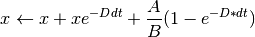
,  is updated according to: