
Getting started with a new library or framework can be daunting, especially when presented with a large amount of reference material to read. This chapter gives a very quick introduction to dana without covering any of the details.
Begin by importing the dana package:
>>> from dana import *
and create a new group of 100 units with a set of definitions:
>>> G = zeros(100,'''r; theta;
                     x = r*sin(theta)
                     y = r*cos(theta)''')
Those definitions represent the underlying model of the group that can be evaluated by invoking the Group.run() method. Let us now affect some random values to r and theta:
>>> G.r = np.random.random(100)
>>> G.theta = 2*np.pi*np.random.random(100)
If we run the group for exactly one iteration, x and y fields will be updated according to their respective definition:
>>> G.run(n=1)
We can display some x and y values of the group:
>>> x,y,r,theta = G.x[0], G.y[0], G.r[0], G.theta[0]
>>> print r, theta
0.496258902417 2.8709367177
>>> print x, y
0.132681542455 -0.478192959504
And check they are equal to their definition:
>>> print r*np.sin(theta), r*np.cos(theta)
0.132681542455 -0.478192959504
Groups are the central objects of the DANA framework and most of the modeling work relates to the definition of a group model which is a set of generic definitions of variables. Such definitions can be a simple declaration of a new variable, an equation defining how to compute the variable (with regards to other variables) or a differential equation defining how to update the variable at each timestep. Let us for example consider the case of a uniform accelerated solid (dx/dy = v, dv/dt = a). Considering the initial state (x₀, y₀) we can easily compute the exact solution x(t) = ½ a.t² + v₀t + x₀.
Simulating such a simple system using DANA is straightforward:
>>> x0, v0, a = 1.0, 2.0, 3.0
>>> t, dt = 1.0, 0.01
>>> G = zeros(1, 'dx/dt=v; dv/dt=a')
>>> G.x, G.v = x0, v0
>>> t,dt = 1.0, 0.01
>>> run(t=t, dt=dt)
>>> print G.x[0]
4.485
And we can check the difference with the theoretical solution:
>>> print 0.5*a*t**2 + v0*t + x0
4.5
The error comes from both the numerical integration and the default integration method which is the forward Euler.
So far, DANA is not very different from (a quite primitive) integration tools allowing for the numerical integration of a set of equations and differential equations. However, one of the strenght of DANA is the possibility to connect groups together allowing them to interact in possibly tricky ways.
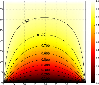
Let us consider for example the heat equation which describe the distribution of heat (or variation in temperature) in a given region over time. For a function u(x,y,t) of two spatial variables (x,y) and a time variable t, the heat equation is given by ∂u/∂t = κ∇²u where κ is a constant. The numerical solution can be approximated using various methods such as the explicit, implicit or Crank-Nicolson methods. We’ll use the explicit method in our implementation and write the heat equation using the forward difference/central difference (FCTS) equation:
>>> n = 50
>>> k = 5
>>> G = dana.zeros((n,n), 'dV/dt = k*(N/4-V); N')
We can connect this group to itself such that each group unit is connected to its four neighbours:
>>> K = np.zeros((3,3))*np.NaN
>>> K[0,1] = K[1,0] = K[1,2] = K[2,1] = 1
>>> print K
[[ nan  1. nan ]
 [  1. nan  1. ]
 [ nan  1. nan ]]
>>> SparseConnection(G('V'), G('N'), K)
The group field N now represents the weighted sum of neighbouring activities. Now, we can simulate the model for ten minutes , keeping left, right and up border at temperature 1 while bottom border is kept at temperature 0.
>>> t, dt = 600.0, 0.1
>>> for i in range(int(t/dt))):
...     G.evaluate(dt=dt)
...     G.V[0,:] = 0
...     G.V[:,n-1] = G.V[n-1,:] = G.V[:,0] = 1
And we can observe the final temperature on the figure below:
The examples presented in this chapter should have given you enough information to get started writing simple simulations.
The remainder of this book goes into more technical details regarding some of DANA’s features. While getting started, it’s recommended that you skim the beginning of each chapter but not attempt to read through the entire guide from start to finish.
There are also numerous examples of DANA applications in the examples/ directory of the documentation and source distributions. Keep checking http://dana.loria.fr/ for more examples and tutorials as they are written.