
A connection can be made between two groups (a source and a target that can be the same) in order to model the propagation of activity from one group to the other. Any connection is evaluated prior to the target group evaluation such that the output of the connection is made available within the group equations.
Creating a connection C between a source and a target using a specified kernel is straightforward:
>>> source = np.ones((2,2))
>>> target = np.ones((3,3))
>>> kernel = np.ones((target.size,source.size))
>>> C = Connection(source,target,kernel)
C now represents the connection between source and target and we can get C output by calling the output function:
>>> print C.output()
[[ 4.  4.  4.]
 [ 4.  4.  4.]
 [ 4.  4.  4.]]
This output is computed by multiplying the source vector by the matrix kernel. However, in the example above, the source is not a vector but a matrix of shape 2×2. To be able to carry out the multiplication, this source is thus flattened into a vector of dimension 4 (= 2×2) and multiplied by the kernel matrix. Since the size of the kernel matrix is 9×4, the output should be a vector of dimension 9. But we know the target group, and more specifically, we know its shape. The output of the connection is thus automatically reshaped such that the shape of the connection output match the shape of the target (3×3 in this case).
The automatic reshaping of the output is critical if it is to be used within a group equation. But before even creating a connection between two groups, we have to decide which field of the target group will receive the output of the connection. This field should be specified as a Declaration as in the following example where field I of target is supposed to receive the connection output.
>>> source = np.ones((2,2))
>>> target = zeros((3,3), 'V = I; I')
>>> kernel = np.ones((target.size,source.size))
>>> C = Connection(source, target('I'), kernel)
We could display the result as it has been made in the previous example the connection output but instead, we’ll use the propagate method that first compute the output of the connection and then store the result within the specified field of the target (I in this case):
>>> C.propagate()
>>> print target.I
[[ 4.  4.  4.]
 [ 4.  4.  4.]
 [ 4.  4.  4.]]
The most interesting point of suchconnections where the target is a group is that the output can be used within the group equations:
>>> source = np.ones((3,3))
>>> target = zeros((3,3),'V = V+I; I')
>>> kernel = np.eye(9)
>>> C = DenseConnection(source, target('I'), kernel)
In this example, the value of V is computed by adding I to the current value. If we run this simple model for 5 iterations, we get:
>>> run(n=5)
>>> print target.V
[[ 5.  5.  5.]
 [ 5.  5.  5.]
 [ 5.  5.  5.]]
A group does not have a topology per se. Even if a shape is specified at group creation, this is mainly used to display it, either on terminal or in a figure. In all of the above examples, we created connections using the full matrix of weights (kernel) specifying individual weight between any source and target unit without further consideration on any possible neighborhood relationship. However, a group may acquire some topology when connected with another group (or itself) if the given kernel has a different shape as illustrated below:
>>> source = np.ones((3,3))
>>> target = np.ones((3,3))
>>> kernel = np.ones((3,3))
>>> C = Connection(source, target, kernel)
>>> print C.output
[[ 4.  6.  4.]
 [ 6.  9.  6.]
 [ 4.  6.  4.]]
Note
It is possible to have toric connections by specifying toric=True when Connection is created
In this case, the given kernel is interpreted as a prototype kernel for a single target unit that is to be used for every other unit. To do this, when the connection is created, a new matrix is built such that any target unit receives the output of the prototype kernel multiplied by the source unit and its immediate neighborood (that span the kernel size) as illustrated on the figure below.
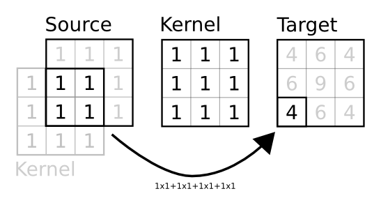
The figure shows how the output of target unit at position (2,0) is computed according to the prototype kernel. First, the shape of the target is used to assign a set of normalized coordinates to the unit and these normalized coordinates are used to find the corresponding source unit. The prototype kernel is then centered on this unit and a element wise multiplication is performed where kernel and source overlaps they are sumed up and stored at the target unit position within the target group. When source and target have the same shape, this is strictly equivalent to a convolution.
All built-in dana connections are built on the same principles but you are free to give the full connection matrix of create your own Connection class to override this behavior.
dana offers three different types of connections that have different properties and speed (for evaluating them). In the following, we’ll consider a source group of size 2×2 and a target group of size 2×2 and a kernel of size 1×1:
>>> source = np.ones((2,2))
>>> target = np.ones((2,2))
>>> kernel = np.ones((1,1))
This is the more generic connection. The underlying matrix is a regular numpy array of size (target.size, source.size). If your two groups are fully connected with no regular patterns in links, you have to use this type of connection:
>>> C = DenseConnection(source,target.kernel)
>>> print C.weights
[[ 1.  0.  0.  0.]
 [ 0.  1.  0.  0.]
 [ 0.  0.  1.  0.]
 [ 0.  0.  0.  1.]]
If you have only a few connection between two groups, you might consider using this type of connection that is built on top of scipy sparse matrix that saves a lot of unnecessary computations when a matrix is mainly filled with zeros:
>>> C = SparseConnection(source,target.kernel)
>>> print C.weights
(0, 0)        1.0
(1, 1)        1.0
(2, 2)        1.0
(3, 3)        1.0