Beyond the quite limited group dtype argument, a group can also be created using a Model that allow to finely tune the behavior of each field of the group. Let us consider the following example:
>>> import Image
>>> image = np.asarray(Image.open('lena.jpg'))/256.0
>>> I = image.view(dtype=[('r',float), ('g',float), ('b',float)]).squeeze()
>>> G = dana.Group(I.shape,
                   model = '''r; g; b; l = 0.212671*r + 0.715160*g + 0.072169*b''')
>>> G.r, G.b ,G.b = I.r, I.g, I.b
G is now a group with 3 regular fields (r, g and b) and a fourth one (l for luminance) that has been defined as a function of the three other fields. If one wants to compute the output of this specific field, one has to simply run the group:
>>> G.run(n=1)
It is to be noted that the l field is not automatically updated when other fields change since we’ll see below that we actually need finer control over evaluation. More generally, a model can be built using either a Declaration, an Equation or a Differential Equation or any combination as described below.
A declaration is a way to declare the existence of a variable to dana. As such, it is not terribly useful when it is used on its own:
>>> eq = Declaration('X')
You can evaluate this declaration by giving the current value of X and quite surprisingly, you get the value of X:
>>> print eq(X=1)
1
When considering a group, a declaration allows to declare the existence of a variable to the group. In this sense, it is quite similar to the dtype syntax where you specify the name of the field and its type. The type of a variable is restricted to scalar types such as bool, int, float and double or any valid numpy scalar types (e.g. np.int32, np.float64, etc):
>>> G = dana.Group((3,3), dtype = [('x', float), ('y', float)])
or (strictly equivalent):
>>> G = dana.Group((3,3), model = 'x : float; 'y' : float')
An equation describes how a given variable is updated when the equation is called. The name of the variable is given by the left-hand side of the equation and the update function is represented by the right-hand side of the equation. Let us consider for example the following equation:
>>> eq = Equation('X = X+1')
It specifies that when equation is called with a X argument, it returns X+1. We can evaluate this equation most simply by making a call to the equation:
>>> print eq(X=1)
2
Of course, you can have more complex equations with many variables and any numpy function:
>>> eq = Equation('X = X+a**2+b')
In such a case, any variables in the right hand side of the equation must be specified when calling the equation. You can choose to name those variables:
>>> print eq(X=1, b=0.1, a=0.5)
1.35
or to specify them in the order they appear in the equation (X,a,b in this case):
>>> print eq(1, 0.5, 0.1)
1.35
Note
Since a and b have not been specified, it is assumed they are equal to zero.
One interesting point is that you can also call the equation with numpy arrays as arguments:
>>> eq = Equation('X = X+2')
>>> print eq(X=np.ones((2,2))
[[ 3.  3.]
 [ 3.  3.]]
A differential equation represents first order ordinary differential equation of the form dy/dt = f(y,t) and describes how a given variable is updated when the equation is called. The name of the variable is given by the left-hand side of the equation and the update function is represented by the right-hand side of the equation. Let us consider for example the following equation:
>>> eq = DifferentialEquation('dX/dt = 1')
Note
Default integration method for differential equations is the forward Euler method.
It specifies that when equation is called with a X argument, it returns X+dX. We can evaluate this equation most simply by making a call to the equation:
>>> X = 1
>>> dt = 0.1
>>> print eq(X,dt)
1.1
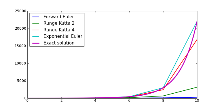
There exists several methods to integrate such differential equation within dana. The fastest is probably the forward Euler method that can give pretty good results as long as your equation is not too stiff as illustrated below (see Wikipedia entry for more informations).

However, if your differential equation is of the form x = A - Bx (which is pretty common in computational neuroscience), you probably better use the exponential Euler integration method that give both fast and accurate results.
If you want to change the integration method, you do it as follows:
>>> eq.select('Runge Kutta 2')
Available methods are:
All the above can now be used in a model that is a container for a set of declaration, equation and differential equations that are evaluated at once when the model is ran. Construction is straightforward:
>>> model = Model('dx/dt = y; y = z+1; z')
Here the model possesses a differential equation (x), an ordinary equation (y) and a declaration (z). This can be checked most easily by printing the model:
>>> print model
DifferentialEquation('dx/dt = Y : float')
Equation('y = z+1 : float')
Declaration('z : float')
To run the model, we need a dictionnary of variables that represent the initial state:
>>> x,y,z = 1,1,1
>>> vars = {'x' : x, 'y' : y, 'z' : z}
We can then use this dictionnay to give the initial state to the model and run it for exactly dt seconds:
>>> model.run(vars, dt=0.1)
{'x': 1.1, 'y': 2, 'z':1}
Warning
Be careful of using distinct numpy arrays for model variables or the result will be undefined.
Instead of scalar variables, you can also use numpy arrays as long as their shape are homogeneous:
>>> x,y,z = np.ones(3), np.ones(3), np.ones(3)
>>> vars = {'x' : x, 'y' : y, 'z' : z}
>>> model.run(vars, dt=0.1)
{'x': array([ 1.1,  1.1,  1.1]),
 'y': array([ 2.,  2.,  2.]),
 'z': array([ 1.,  1.,  1.])}