11. Examples

11.1. Image processing

A lot of standard image processing technics are based upon homogeneous convolution of individual pixels with surrounding regions (Gaussian blur, Sobel operator, Cross operator, etc.). Dana is perfectly suited for such technics offering easy manipulation of kernel functions. We’ll use the Imaging library to load the standard lena image into a numpy array. The shape of the array is either width×height for gray-level images or width×height×[3,4] for color images (RGB or RGBA):

>>> import Image
>>> image = np.asarray(Image.open('lena.png'))/256.0
>>> I = image.view(dtype=[('R',float), ('G',float), ('B',float)]).squeeze()
>>> L = (0.212671*I['R'] + 0.715160*I['G'] + 0.072169*I['B'])

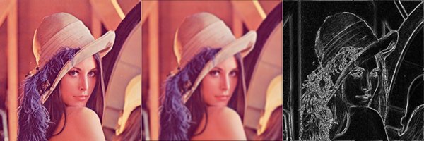
Figure Original lena image, blur filter and Sobel filter.

11.1.1. Sobel operator

The Sobel operator is used for edge detection and is based upon a differentiation operator that approximate the gradient of the image intensity. Technically, this is made using two convolutions (one horizontal and one vertical) with a minimal size kernel (3×3) to get local gradients from which we can compute the gradient magnitude:

>>> src = Group(I.shape, 'V = sqrt(Gx**2+Gy**2); Gx; Gy')
>>> Kx = np.array([[-1., 0.,+1.],
                   [-2., 0.,+2.],
                   [-1., 0., 1.]])
>>> Gx = SharedConnection(L, src('Gx'), Kx)
>>> Ky = np.array([[+1.,+2.,+1.],
                   [ 0., 0., 0.],
                   [-1.,-2.,-1.]])
>>> Gy = SharedConnection(L, src('Gy'), Ky)
>>> src.run(n=1)

11.1.2. Gaussian blur

Gaussian blur is based upon the convolution of the image using a Gaussian kernel. In the example below, we use a 5×5 Gaussian kernel and we apply it on the three channels:

>>> G = gaussian((10,10),.5)
>>> K = G/G.sum()
>>> SharedConnection(I['R'], I['R'], K).propagate()
>>> SharedConnection(I['G'], I['G'], K).propagate()
>>> SharedConnection(I['B'], I['B'], K).propagate()

11.2. Cellular automata

Have a look at the chapter From numpy array to dana group for a commented implementation of the game of life.

11.3. Diffusion process

Have a look at the chapter Quick tour for a commented implementation of a diffusion process.

11.4. Dynamic neural fields

Dynamic neural fields describe the spatio-temporal evolution of a population of neurons seen as a spatial continuum. These models have been extensively studied in [Wilson:1972] , [Wilson:1973], [Amari:1977] and [Taylor:1999] extended these studies in the two-dimensional case. We will use notations introduced by Amari where a neural position is labelled by a vector x.

with

• U(x,t) is the potential of a neural population at position x and time t.
• W(x) is a neighborhood function
• f(x) is the firing rate of a single neuron.
• α is the temporal decay of the synapse.
• h is the resting potential
• I(x,t) is the input at position x

Usually, the neighborhood function W is a difference of Gaussian (a.k.a. Mexican hat) with short range excitations and long range-inhibitions.

We begin by setting simulation parameters:

>>> n = 256
>>> t, dt = 10.0, 0.01
>>> alpha = 1.0

We create the input (I) and neural field groups:

>>> I   = np.zeros((n,))
>>> DNF = Group((n,), '''dU/dt = (-V + 0.1*L + I);
                          V    = maximum(U,0); I; L''')

and we connect the input to the neural field and the neural field to itself:

>>> SparseConnection(I, DNF('I'), np.ones((1,)))
>>> SharedConnection(DNF('V'), DNF('L'), +1.00*gaussian(2*n+1, 0.10)
                                         -0.75*gaussian(2*n+1, 1.00))

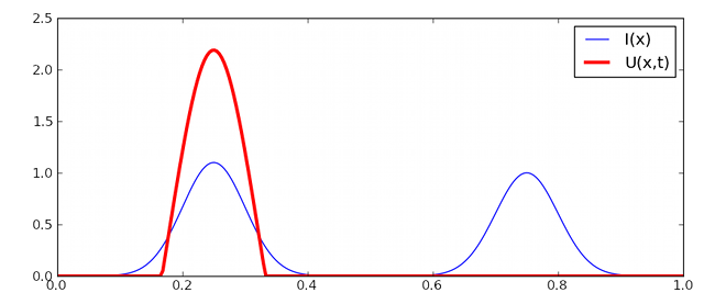
Finally, we setup some input and we run the model:

>>> I[...] = 1.1*gaussian(n, 0.1, -0.5) + 1.0*gaussian(n, 0.1, +0.5)
>>> run(t=10.0, dt=0.1)

11.4.1. References

[Amari:1977]

S.-I. Amari, Dynamic of pattern formation in lateral-inhibition type neural fields, Biological Cybernetics, 27:77-88, 1977.

[Wilson:1972]

H.R. Wilson and J.D. Cowan Excitatory and inhibitory interactions in localized populations of model neurons, Biophysical Journal, 12:1-24, 1972.

[Wilson:1973]

H.R. Wilson and J.D. Cowan. A mathematical theory of the functional dynamics of cortical and thalamic nervous tissue. Kybernetik, 13:55–80, 1973.

[Taylor:1999]

J.G. Taylor Neural bubble dynamics in two dimensions: foundations, Biological Cybernetics, 80:5167-5174, 1999.